Traffic Routing

Matthew Burke

5 min read May 16, 2026

Optimizing Transaction Routing with Linear Programming

A side project exploring cost-minimizing vendor allocation under uncertainty.

---

When you process a large volume of transactions, you’re often not locked into a single vendor. Multiple vendors compete for your volume, each offering tiered pricing, volume commitments, and restrictions on which transaction types they’ll accept. The question becomes: how do you decide where to send each transaction to minimize cost while keeping everyone happy?

This post walks through a two-stage optimization approach to that problem, built using Google’s OR-Tools and a bit of statistics.

---

The Setup

The problem has a few moving parts:

• Vendors each have a minimum and maximum volume they’ll accept, and tiered pricing (the more you send, the cheaper it gets).
• Packet types are different categories of transactions, and not every vendor accepts every type.
• Forecasts for how many transactions of each type you’ll process are uncertain — you have a mean and standard deviation, not a hard number.

The goal: given a volume forecast, allocate transactions across vendors to minimize total cost, while satisfying vendor minimums/maximums and packet type restrictions.

---

Handling Forecast Uncertainty

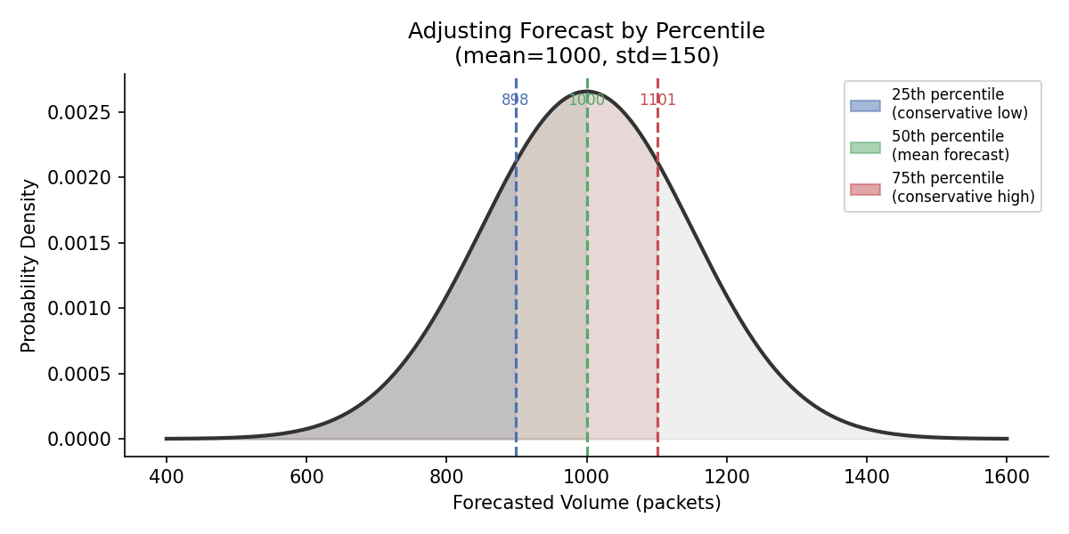
Before optimizing anything, you need a volume to plan against. The ForecastGenerator class handles this and includes a useful lever: rather than just using the mean forecast, you can adjust it to any percentile of the expected distribution.

def adjust_forecasts(self, adjustments: dict) -> None:
    for packet_type, percentile in adjustments.items():
        mean = self.forecast[packet_type]["mean"]
        std_dev = self.forecast[packet_type]["std_dev"]
        self.forecast[packet_type] = self._calculate_adjusted_forecast(
            mean, std_dev, percentile
        )

def _calculate_adjusted_forecast(mean, std_dev, percentile):
    z_score = norm.ppf(percentile)
    return mean + (z_score * std_dev)

So if you want to plan conservatively (protecting against higher-than-expected volume), you pass percentile=0.75 or 0.90. If you’re fine with the base case, use 0.50. This is a lightweight way to bake risk tolerance into the planning process without needing a full simulation.

---

Stage 1: Figuring Out How Much Goes to Each Vendor

The first optimization problem answers: given a total volume, how should we split it across vendors and tiers to minimize cost?

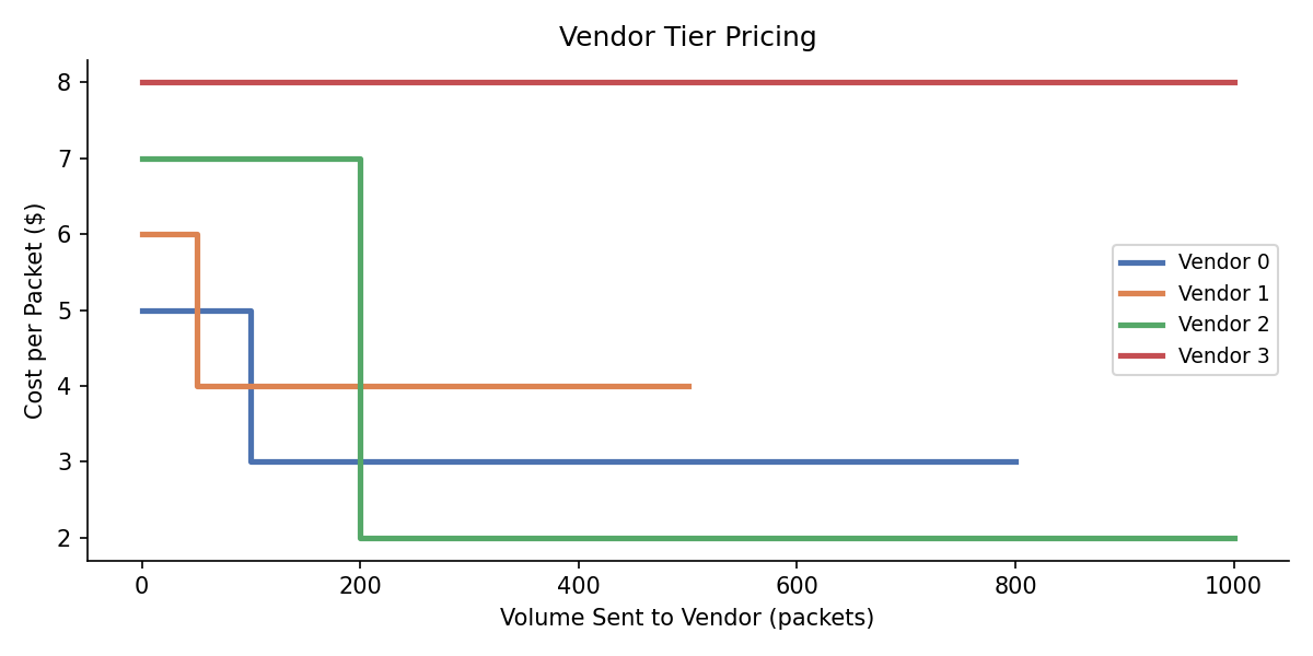
Each vendor has one or more pricing tiers. A tier kicks in after you’ve sent a certain volume — like a bulk discount. The trick is that tiers have to be filled in order; you can’t jump to the cheap tier without meeting the volume threshold for the cheaper tiers first.

Each vendor’s pricing structure looks like this — the solver is incentivized to push volume high enough to unlock the cheaper tiers:

This is a classic integer linear program. The decision variables are the number of packets assigned to each vendor at each tier:

x[vendor][tier] = number of packets at this tier

The objective is to minimize total cost:

minimize: sum over all vendors and tiers of (cost_per_packet[i][j] * x[i][j])

Subject to:

• Total packets shipped equals the forecast
• Each vendor stays within its min/max volume
• Tier volume constraints are respected (you can’t access tier 2 without filling tier 1 first)

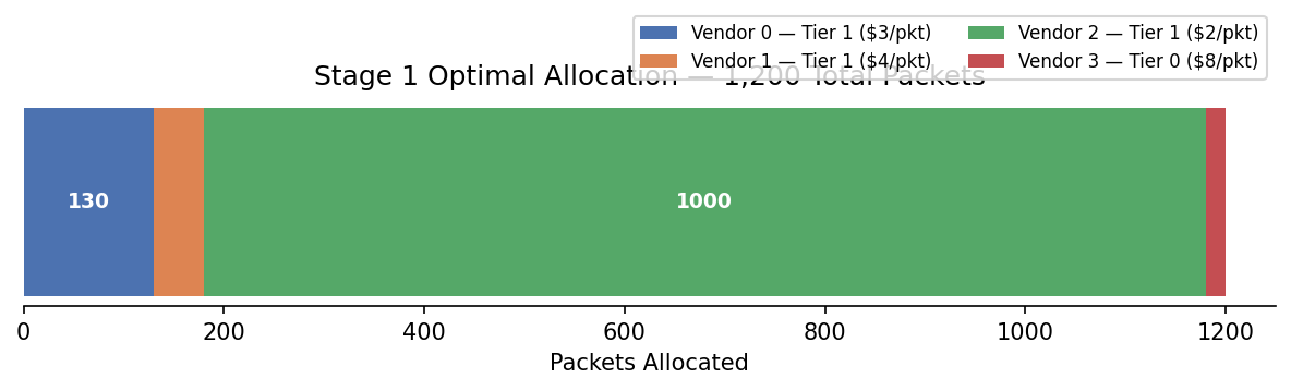
Using OR-Tools’ SCIP solver, this resolves quickly even with several vendors and tiers. A sample run with four vendors and 1,200 total packets looks like:

Vendor 0:  Tier 1: 130 packets
Vendor 1:  Tier 1:  50 packets
Vendor 2:  Tier 1: 1000 packets
Vendor 3:  Tier 0:  20 packets
Total cost = 2750.0

The solver naturally gravitates toward Vendor 2’s deep-discount tier since it has the lowest per-packet cost once the volume threshold is met.

The output from this stage isn’t just volumes — it’s also the effective cost per packet for each vendor, which becomes the input to Stage 2.

---

Stage 2: Routing Each Packet Type

Now comes a subtler problem. Not all packet types can go to all vendors. So knowing “send 1,000 packets to Vendor 2” isn’t enough — you need to know, for each packet type, what fraction to route where.

The PacketRouteOptimizer solves this. Decision variables are the routing fractions:

x[packet_type][vendor] = fraction of this packet type sent to this vendor

If a vendor doesn’t accept a packet type, its variable is locked to 0. Otherwise it’s a continuous variable between 0 and 1.

The objective is again cost minimization:

minimize: sum over all packet types and vendors of
          (volume[packet_type] * cost[vendor] * x[packet_type][vendor])

With constraints that:

• Every packet type’s fractions sum to 1 (all packets get shipped)
• Each vendor receives at least its minimum committed volume across all packet types

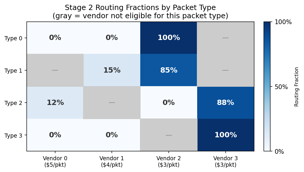
A sample result with four packet types and four vendors:

Package Type 0:  Vendor 2: 100.00%
Package Type 1:  Vendor 1: 15.00%,  Vendor 2: 85.00%
Package Type 2:  Vendor 0: 12.50%,  Vendor 3: 87.50%
Package Type 3:  Vendor 3: 100.00%
Total cost = 4030.0

The solver routes as much as possible to the cheapest eligible vendor for each packet type, then uses secondary vendors only as much as needed to satisfy commitments.

---

Translating Fractions to Runtime Routing

The optimization outputs fractions — but at runtime, when a transaction arrives, you need to make a concrete routing decision. The VendorRouter handles this using a cumulative probability approach.

def _prepare_cumulative_fractions(self) -> None:
    cumulative_fractions = []
    cumulative_vendors = []
    fraction = 0
    for vendor, v_fraction in self.vendor_fractions.items():
        fraction += v_fraction
        cumulative_fractions.append(fraction)
        cumulative_vendors.append(vendor)

def get_vendor(self, fraction: float) -> Vendor:
    for i, cum_fraction in enumerate(self.cumulative_fractions):
        if fraction <= cum_fraction:
            return self.cumulative_vendors[i]
    return self.cumulative_vendors[-1]

You pass in a random float between 0 and 1 (from a hash of the transaction ID or a random draw), and it maps to the appropriate vendor based on the cumulative distribution. For the example above where Vendor 2 gets 85% of Package Type 1: any draw below 0.15 goes to Vendor 1, anything else goes to Vendor 2. Clean and deterministic if you use a hash.

---

How It Fits Together

The full pipeline looks like this:

1. Forecast — load mean/std_dev forecasts per packet type and adjust to your desired percentile
2. Price tier optimization — find the optimal vendor volume split to minimize cost, accounting for tiered pricing and commitments
3. Route optimization — given per-vendor costs and per-packet-type restrictions, find the fractional routing that minimizes cost while meeting vendor minimums
4. Runtime router — load the fractional routing into a PacketRouter and use it to make live routing decisions

The two optimization stages are deliberately separate. Tier pricing depends only on total volume per vendor. Routing fractions depend on per-packet-type restrictions and the per-vendor cost outcomes from Stage 1. Decoupling them keeps each problem tractable.

---

Wrapping Up

This was a fun use case — it sits at the intersection of forecasting, combinatorial optimization, and systems design. OR-Tools made the LP formulation straightforward, and the stats-based forecast adjustment adds a practical handle for managing risk without overcomplicating the model.

A few obvious directions to extend this:

• Multi-period optimization: run this weekly or monthly and account for volume rollover across periods
• Stochastic programming: instead of picking a single percentile, optimize over a distribution of forecast scenarios
• Dynamic repricing: re-optimize routing mid-period if actual volume deviates significantly from forecast

The code is available on GitHub if you want to dig in.