

In the first version of this project, I built a Codenames spymaster assistant using word embeddings and cosine similarity. It worked okay, but I called out the main weakness at the end: embeddings struggle with polysemy, proper nouns, and anything that requires a concrete, verifiable connection between words rather than a vague semantic cloud. I said graph-based similarity would fix that, and I finally got around to building it.
This post covers three approaches — a Wikipedia link graph via Neo4j, a pure LLM approach using Gemini, and the original GloVe baseline — alongside a real evaluation loop using the SALT-NLP dataset of human-labeled Codenames games. The code is on GitHub.
The headline result: the graph approach is fast, auditable, and free at runtime — but it has a structural yield gap I couldn’t close with graph tuning alone. And the pure LLM approach, despite its limitations, just works.
Three Approaches at a Glance
Before going deep, here’s how the three generators compare across the dimensions that matter for this problem:
| Graph (Neo4j) | Pure LLM (Gemini) | GloVe | |
|---|---|---|---|
| Yield | 68% | ~100% | 86% |
| Avg latency | 40ms | 2–5s | 12ms |
| Precision@K | 0.941 | TBD | 0.965* |
| Legality guarantee | Strong | Weak | Medium |
| Handles polysemy | No | Yes | Partially |
| Infrastructure | Neo4j + Docker | API key only | GloVe model file |
| Cost per request | ~$0 | ~$0.002–0.005 | $0 |
GloVe Precision@K is inflated — the SALT dataset stores team words as targets, so any generator that returns team words scores near 1.0. Take that number with a grain of salt.
The Graph Pipeline
The core idea: two Codenames words are related if they share Wikipedia neighbors. If SHARK and OCEAN both link to the Wikipedia article for “Marine biology,” then “marine” is a candidate clue connecting them. The more team words a candidate connects, the better.
The pipeline looks like this:
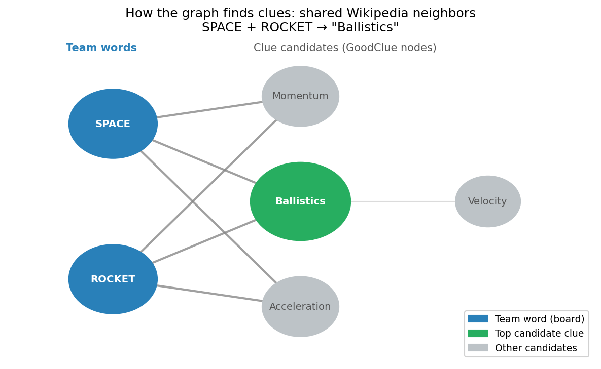
How the graph finds clues: SPACE and ROCKET both link to the Wikipedia article for “Ballistics”, making it a candidate clue. The generator scores all such shared neighbors across every team word pair.
A quick primer on graph databases
If you haven’t worked with a graph database before, the core idea is simpler than it sounds. Where a relational database stores data in tables (rows and columns), a graph database stores data as nodes (things) and edges (relationships between things). That’s it.
For Wikipedia: every article is a node, and every hyperlink from one article to another is an edge. The full English Wikipedia graph has ~13.6 million nodes and hundreds of millions of edges.
Querying a graph database works by pattern matching — you describe the shape of the data you want, and the database finds all subgraphs that match. In Cypher (Neo4j’s query language), (a)--(b) means “find node a connected to node b by any edge.” You can chain these: (a)--(b)--(c) finds any path of length two. No joins, no subqueries — just describe the shape.
So “find all Wikipedia articles that both SPACE and ROCKET link to” is literally:
(space_node)--(candidate)--(rocket_node)
That’s the entire structural logic of the clue generator. Everything else is filtering and scoring on top of that pattern.
Building the graph
The Wikipedia link graph lives in Neo4j. The first step on each request is mapping board words to Wikipedia page titles via an indexed UNWIND lookup:
UNWIND $words as w
MATCH (p:Page)
WHERE p.title = w
   OR p.title = toUpper(substring(w, 0, 1)) + substring(w, 1)
   OR p.title = toUpper(w)
RETURN p.title as title, w as lower_title
This runs in under 5ms. The first version used toLower(p.title) IN $words, which forced a function call on every node and bypassed the index — triggering a full scan of 13 million nodes that took 24 seconds. The UNWIND pattern with explicit equality checks hits the index on every lookup.
Finding candidates with GoodClue nodes
Not every Wikipedia page makes a good Codenames clue. “List of mammals by country” is technically connected to a lot of things, but it’s useless. To avoid polluting the candidate set, I precomputed a GoodClue label on nodes that pass a degree filter (200–10,000 links) and title pattern filters (no “List of”, no taxonomy suffixes, no linguistics meta-articles). This runs once offline via precompute_graph.py and takes about 12 minutes for ~950k nodes.
At query time, finding candidates is the pattern match described above, with filters:
MATCH (team:Page) WHERE team.title IN $team_words AND team.degree < 5000
MATCH (candidate:GoodClue)--(team)
WHERE NOT candidate.title IN $team_words
WITH candidate, collect(DISTINCT team.title) AS targets
WHERE size(targets) > 1 OR $team_words_count < 3
ORDER BY candidate.base_score DESC
LIMIT 150
In plain English: find all GoodClue nodes that are neighbors of at least two team-word nodes, collect which team words each candidate connects, and return the top 150 by precomputed score.
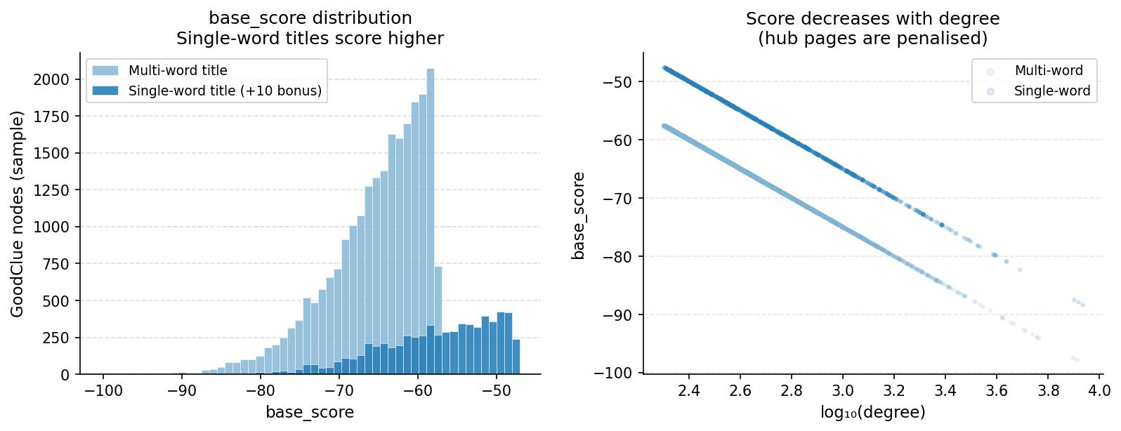
base_score is precomputed as -log10(degree) * 25 + 10 (single-word bonus). Pages with middling degree get the highest scores — they’re specific enough to be useful, but connected enough to bridge multiple team words. The distribution across all 950k GoodClue nodes shows the two-population effect clearly: single-word titles cluster above the multi-word titles by exactly the +10 bonus.
The scoring pass runs after the LIMIT 150 to avoid computing opponent/neutral overlaps on thousands of candidates:
WITH candidate, targets,
     [(candidate)--(opp:Page) WHERE opp.title IN $opp_words | opp.title] AS opp_targets,
     [(candidate)--(neut:Page) WHERE neut.title IN $neut_words | neut.title] AS neut_targets
RETURN candidate.title AS clue, targets,
       (base_score + size(targets)² * team_weight
                   - size(opp_targets) * opp_penalty
                   - size(neut_targets) * neut_penalty) AS score
ORDER BY score DESC LIMIT 50
Making It Fast
The first working version had an average latency of 4.9 seconds, with a worst case of 32 seconds for boards with high-degree words like “gold” or “lead.” The fix was three changes applied together:
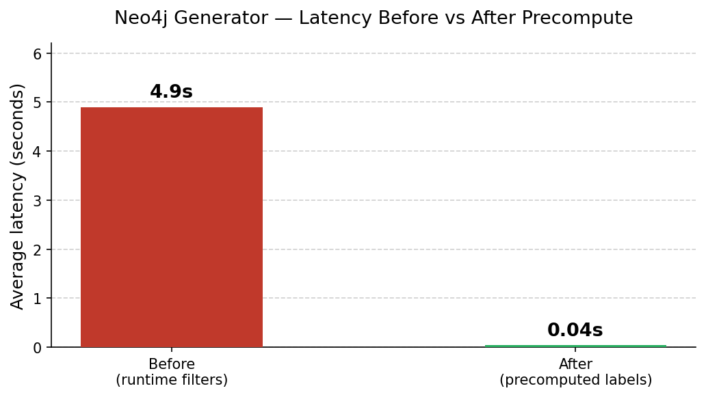
Before and after latency. The 32-second outliers disappeared entirely.
-
Precompute
GoodCluelabels andbase_scoreoffline. The runtime query was running 13 title-pattern filters and computing a log-degree penalty on every candidate on every request. Moving this to a one-time precompute step made the runtime query trivially cheap. -
Add
LIMIT 150before the scoring pass. The opponent/neutral overlap subqueries are expensive and were running on thousands of candidates. Limiting to the top 150 bybase_scorefirst makes the scoring pass fast without meaningfully affecting result quality. -
Lower the team degree cutoff from 10,000 to 5,000. Words like “gold” (degree ~7,600) were triggering full neighborhood traversals. Filtering them out at the team-word stage — not the candidate stage — cuts the graph traversal early.
Optional AI Layers
With the graph running fast, I added two optional re-ranking steps that activate when a Google API key is provided:
Gemini Embedding Reranker — embeds the clue and all target words using gemini-embedding-001, then adds two signals: average clue-to-target cosine similarity (does the clue actually relate to the targets semantically?) and target cluster tightness (are the targets themselves a coherent group?). The graph can surface a clue like “Cladistics” that technically connects BIRD and FISH through Wikipedia, but the embedding reranker penalizes it because the connection is obscure.
LLM Scorer — sends the top 20 candidates to Gemini Flash and asks it to rate each one 1–10 on naturalness. The rating is folded into the composite score as a continuous term rather than a binary filter. This catches Wikipedia-jargon clues that the graph scores highly but no human would ever use in a game.
One practical note on API quota: the free tier for Gemini Flash has per-minute and daily limits. To handle this without interrupting runs, all LLM calls go through a fallback chain that tries models in order — gemini-2.5-flash-lite → gemini-2.5-flash → gemini-2.0-flash-lite → gemini-2.0-flash — skipping to the next on any 429 or quota error.
Evaluating Against Real Games
The SALT-NLP dataset contains human spymaster clues for real Codenames boards, which makes it a useful benchmark. I ran all three generators against 50 SALT scenarios and tracked four metrics:
- Yield: fraction of scenarios that produced at least one clue
- Precision@K: how well the top clue’s targets match the human clue’s targets
- SingleWord rate: fraction of top clues that are plain alphabetic words (proxy for legality)
- Avg latency: generation time per scenario
| Generator | Yield | Precision@K | SingleWord | Avg latency |
|---|---|---|---|---|
| Neo4j | 34/50 (68%) | 0.941 | 66% | 0.040s |
| Semantic (GloVe) | 43/50 (86%) | 0.965* | 86% | 0.012s |
GloVe Precision@K inflated — see note above.
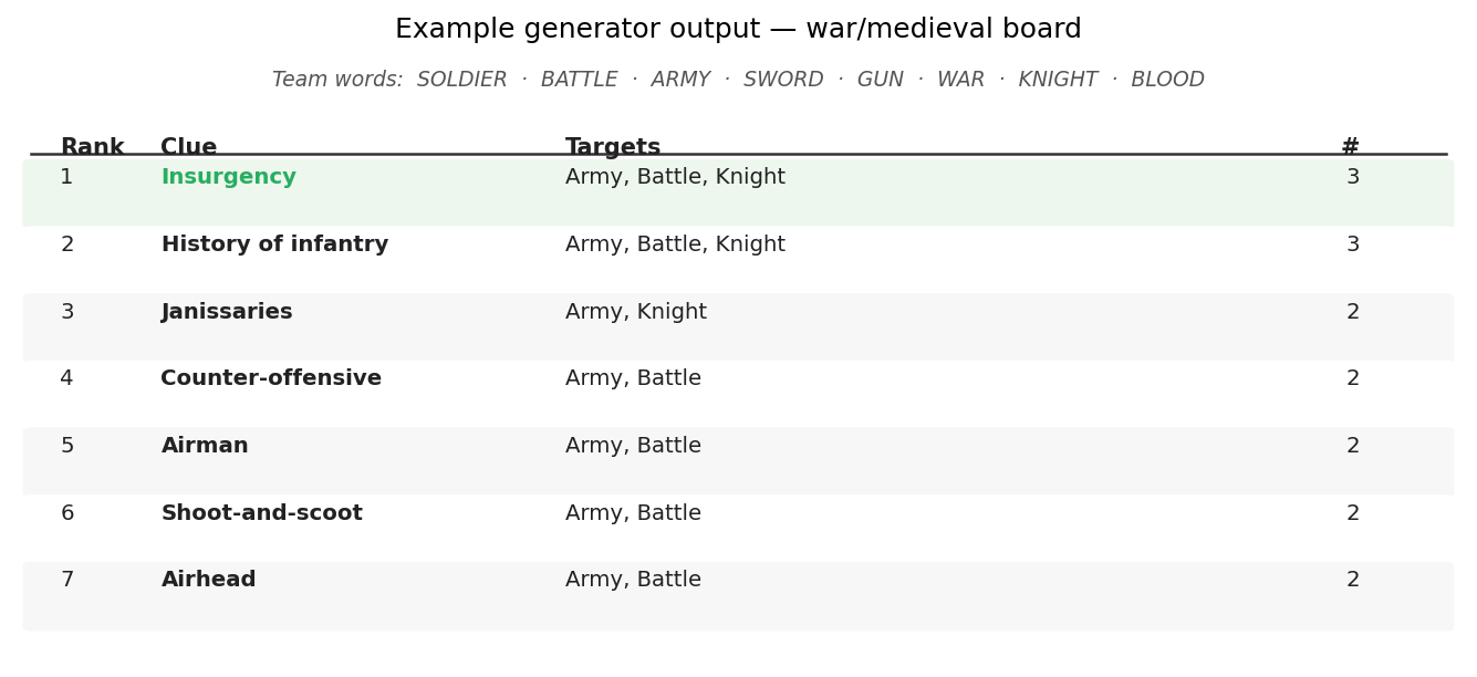
To make this concrete, here’s what the generator actually returns for a war/medieval-themed board:
The Yield Gap: What I Got Wrong
The 32% yield gap bothered me. My assumption was that this was a word-mapping problem — board words like “sub” or “boom” weren’t matching Wikipedia titles, so the graph had nothing to work with.
To test this, I built a WikipediaWordMapper that uses full-text search on the page_title index, embedding similarity to rank candidates, and an LLM call to disambiguate when the top two matches are close. The idea was that “charge” would resolve to the “Charge” Wikipedia article, “bark” to “Bark (dog)”, and so on.
After wiring it in and re-running the eval: yield unchanged at 68%.
Digging into the failing scenarios revealed the actual problem. The failing board words do map via the initial UNWIND lookup — “sub” resolves to the “Sub” Wikipedia article just fine. The issue is what happens next:
| Word | Wikipedia title | Degree | GoodClue neighbors found |
|---|---|---|---|
| sub | Sub | 40 | 0 |
| boom | Boom | 100 | 0 |
“Sub” has 40 Wikipedia links total. None of its neighbors are GoodClue nodes (which require degree 200+), so the graph query returns no candidates. The WikipediaWordMapper can’t help here — the word mapped, it just mapped to a page with sparse connections.
I tried lowering the GoodClue floor from degree 200 down to 50, which added ~200k new candidate nodes. Results: zero yield improvement, average latency increased 13x (40ms → 520ms), and the single-word rate dropped because the new low-degree nodes tend to have multi-word Wikipedia titles. Reverted.
The 32% gap is structural for this dataset. Many SALT scenarios involve words that genuinely have thin Wikipedia footprints — they’re common English words, but their Wikipedia pages are stubs or disambiguation pages with few meaningful connections. The graph has nothing to bridge from.
The Pure LLM Approach
Given the yield gap, I added a pure LLM baseline: send the full board to Gemini with a prompt asking for the best clues, parse the JSON response.
prompt = f"""You are an expert Codenames spymaster. Generate the best clues for the board below.

YOUR team words: {', '.join(w.upper() for w in my_team)}
Opponent words (avoid): {', '.join(w.upper() for w in opponent)}
Neutral words (avoid): {', '.join(w.upper() for w in neutral)}
Assassin (instant loss if guessed): {assassin.upper()}

Return ONLY valid JSON — a list of up to 10 clues, best first:
[{"clue": "WORD", "targets": ["word1", "word2"], "justification": "brief reason"}]"""
The LLM handles polysemy naturally (it knows BANK means money in a financial context), generates clues humans would actually use, and has 100% yield by definition. The tradeoffs: 2–5 second latency, no verifiability, and the occasional hallucinated connection.
Recommendation
If you want a Codenames clue generator that works and you’re willing to pay a fraction of a cent per request, use the LLM approach. It has 100% yield, produces natural clues, handles proper nouns and slang, and requires nothing beyond an API key. LLMs are increasingly just solving this class of problem — structured reasoning over a constrained set of words is exactly what they’re good at.
The graph approach is worth building if you care about why a clue is connected — you can trace exactly which Wikipedia articles link a clue to a team word, which is useful for understanding and tuning the system. It’s also genuinely fast (40ms with no API calls) and free at runtime after the Neo4j setup cost. But the yield gap means you’d want to pair it with an LLM fallback for boards where the graph comes up empty.
For most people: prompt the LLM, ship it.
What’s Next
A few obvious directions:
- LLM fallback for zero-candidate boards — run the graph first; if it returns nothing, fall back to LLM-Direct. Gets yield close to 100% while keeping the graph path for the majority of boards where it works
- Stricter eval metric — current Precision@K measures target word overlap, which is inflated for some generators. Comparing the generated clue word to the human clue word is a harder and more honest measure
- Grid tuning — the scoring weights (
team_weight,opp_penalty,neut_penalty) haven’t been systematically tuned yet.evaluation_framework.py+grid_tuner.pyare ready to run once the eval metric is trustworthy
Side note: managing free-tier API quota
One thing that came up repeatedly during development: the Gemini free tier has both per-minute (RPM) and daily (RPD) limits, and they’re easy to exhaust when running evaluations in a loop.
Running 50 eval scenarios back-to-back with LLM-Direct active burned through the daily gemini-2.0-flash-lite quota in a single run. The per-minute limits are just as easy to hit — 15 RPM means a 50-scenario eval takes at least 3–4 minutes minimum even if each call is fast.
A few things that helped:
Build a fallback chain, not a single model reference. Instead of hardcoding a model name and getting a hard failure on quota exhaustion, keep an ordered list and retry down it on any 429 or RESOURCE_EXHAUSTED error:
FLASH_FALLBACK_MODELS = [
    "gemini-2.5-flash-lite",   # highest free-tier RPD
    "gemini-2.5-flash",
    "gemini-2.0-flash-lite",
    "gemini-2.0-flash",
]
This way a quota exhaustion on one model silently rolls to the next rather than crashing the run. You lose nothing on the happy path and gain resilience on the quota-hit path.
Probe availability before a long run. A quick /quota-check at the start of a session — hitting each model with a single cheap request and checking for 429s — tells you which models are available before committing to a 50-scenario eval. Saves the frustration of a run failing 40 scenarios in.
Different models have different daily limits, not just rate limits. The per-minute limits are well-documented, but the daily limits are less predictable and reset at midnight Pacific. If you’re hitting daily limits, spreading eval runs across days or using a paid tier is the cleaner solution than trying to optimize around the caps.