


Multi-Armed Bandit Overview
A multi-armed what?? If you don’t know what the multi-armed bandit problem is, then you may be confused. I’m assuming that you have some background on this for the rest of the post, but if you don’t, here’s a quick rundown:
Pretend you are a someone who’s looking to go gambling, and an old style slot machine (aka bandit, don’t worry about why) you can choose from that has multiple arms. Your goal is (obviously) to make the most amount of money from putting coins into it and pulling the arms. However, given that you can only try one arm at a time, how do you find the arms(s) that give you the most bang for your buck without wasting time on arms that just eat your money?
That’s essentially what the multi-armed bandit problem is. How do we maximize rewards by exploring new arms we don’t know much about (have only played zero or a few times), while still exploiting (or taking advantage of) the arms we already know give us good rewards?
Alright, now that we’ve covered that, we can jump into some code and ways I explored common algorithms used to maximize profits in this scenario.
Bandit Definitions
But first, let’s look again at how the bandits themselves are defined. I played around with two types:
- Bernoulli Bandit: each arm in the bandit has a set probability each time it’s pulled of returning a reward of 1 or 0
- Gaussian Bandit: each arm in the bandit has a mean and standard deviation that define a gaussian distribution. When pulled, it samples from that distribution to return a reward.
Here’s a quick visualization of means and a standard deviation away from those means to get an idea of the potential overlap in rewards you may get from the gaussian bandits. The x axis is the arm number, and the y axis is the reward distribution.
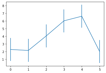
Clearly arms 3-4 are the highest ones, but their rewards still overlap greatly with 2, and it would be tricky to tell which one is best, given the amount of noise when sampling.
Execution
The methods to choose arms in a programmatic away could be called methods or algorithms or whatever, but since I’ve been exploring reinforcement learning recently, I’m going to call them agents.
At each timestep a few things happen:
- The agent evaluates its current stored information and chooses an arm to interact with
- The agent pulls the chosen arm and receives a reward in return
- The agent makes updates to its stored information based on the reward
The parts where the different methods differ is mainly in step 1, where they use different methods to choose the arm. Step 3 supports step 1 by updating the stored information, and is similar across most agents with some minor differences.
Evaluation Procedure
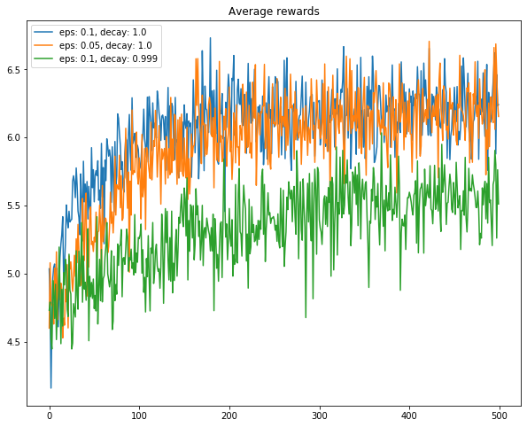
In the following section, I compare agents with different parameters to each other by running an agent against a bandit for a pre-defined number of timesteps repeatedly. By doing this multiple times and tracking the rewards at each timestep, we can get a sense of what average performance we can expect from the agent at each timestep.
Naturally, we should see lower average rewards earlier on since we are still exploring and are uncertain of which arms provide the best value, but what we hope to see is a gradual increase in rewards until we identify the optimal arm, at which point the rewards should flatten out to the average of the optimal arm’s reward.
The two plots I include each with the comparisons track both of the metrics over time:
- Average reward at each timestep
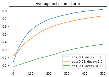
- Percent of times the agent chose the optimal arm at that timestep
As you will see, the former can be a rather noisy chart (especially with gaussian reward functions), but the latter results in a smoother chart.
Agents
Epsilon Greedy
The epsilon greedy agent is an agent is defined by two parameters: epsilon and epsilon decay.
Every timestep, in order to select the arm to choose, the agent generates a random number between 0 and 1. If the value is below epsilon, then the agent selects a random arm. Otherwise, it chooses the arm with the highest average reward (breaking ties randomly), thus exploiting what it knows.
A higher epsilon results in more exploration (random arm selections), and a lower epsilon results in more exploitation.
Because we may not want to keep the same epsilon over the life of our problem, we introduce the epsilon decay parameter, which decreases the value of epsilon after each timestep. This naturally lends itself towards a high explore approach at the beginning when we are unsure of the arm rewards, and a high exploit approach later on once we have more information.
In theory, this seems like a good idea, but in practice (with noisy rewards), decaying epsilon seems to have slightly lower performance. However, I did not implement a minimum epsilon, which could help by preventing a fully-exploit scenario.
Below is a comparison of some different parameters of epsilon greedy agents:
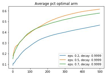
Here is a comparison of the best decay rate I found (ratio of 0.9999 per timestep) with different starting epsilon values.
UCB
The upper confidence bound (UCB) agent tracks the average reward for each arm similar to epsilon greedy, but rather than encoding its exploration as a binary random chance, it attempts to measure uncertainty in terms of how long it has been since a arm has been chosen.
Each timestep, the agent chooses the arm with the highest average reward plus “uncerainty”, and the uncertainty for each arm not chosen increases a little bit.
Earlier on, every timestep where a arm is not chosen increases uncertainty by a significant amount. As the system time grows, the uncertainty contributed by each timestep decreases since we should have more accurate estimates of rewards as time progresses.
An important note is that this uncertainty is not what we normally think of in statistics and is not related to the variance of the reward estimates.
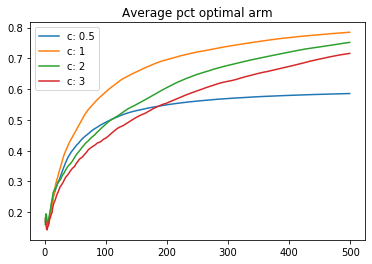
The influence of the uncertainty factor is determined by a parameter C. Below is a comparison of some runs with different values of C:
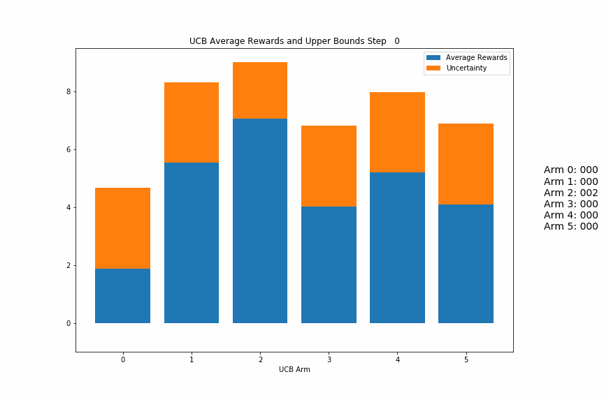
One of the main purposes of this repo was to help visualize the UCB agent, in terms of how it balances the average rewards received so far and the uncertainty of unused arms.
Below is as gif of a UCB agent in action. Each frame in the gif is a step where the agent chose an action, received a reward, and updated its estimates/uncertaintities for each arm.
The blue parts of each bar are the average rewards for that arm, and the orange parts are the uncertainty. You should be able to see the blue parts jump around as the highest total blue + orange arm is pulled, while the non-pulled arms’ orange parts should steadily increase until they become the highest bars.
At first, the values will most likely jump around more as the variance of the reward estimates is large, but as it progresses, it should settle into selecting a few arms repeatedly until there is one main winner.
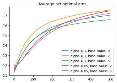
Gradient Method
The prior two algorithms choose arms based on the average score values, selecting the highest performing one (with some initial exploration). Gradient-based algorithms instead relies on relative preferences for each arm that do not necessarily correspond to actual rewards values. At each timestep, the rewards for an arm are observed, and then an incremental update to the existing preference score is made based on new score and a parameter alpha. This is similar to stochastic gradient ascent, and a larger alpha will result in a larger step size.
The details for updating the preference values \(H_{t}(a)\) for selection probabilities \(\pi_{t}(a)\) selected action \(A_{t}\), rewards \(R_{t}\), and average reward \(\overline{R_{t}}\) are as follows:
\(H_{t+1}(A_{t}) = H_{t}(A_{t}) + \alpha (R_{t} - \overline{R_{t}})(1 - \pi_{t}(A_{t}))\) for action \(A_{t}\) and
\(H_{t+1}(a) = H_{t}(a) - \alpha (R_{t} - \overline{R_{t}})\pi_{t}(a)\) for other actions \(a \neq A_{t}\)
When choosing an arm, the agent passes these arm preferences through the softmax distribution to assign weights to all arms that add up to one. These weights are the probabilities that each arm is chosen. After each step, the average rewards are updated, then the weights for sampling are recalculated.
In case you aren’t familiar, the softmax distribution is as follows: \(P\{A_{t} = a\} = \frac{e^{H_{t}(a)}}{\sum_{b=1}^k e^{H_{t}(b)}}\)
One thing to note is that the average rewards at the start before any weights are input affects the results. Starting all arms out with a value greater than zero will still have an effect of an equal chance for all arms to be selected, but will encourage more exploration in the short term before potentially lowering poorly performing probabilities of being selected almost to zero.
Interactive Notebook
I created a github repo with all of the code used to generate these plots, with a notebook ready to to re-run them and change any parameters so you can get an intuition about how some of these common agent algorithms work.
I’d highly recommend playing around with different numbers of arms, bernoulli rewards, and various levels of noise in the gaussian rewards by increasing and decreasing the standard deviation compared to the means.