PyMC Wrapper

Overview

Bayesian modeling can be super valuable for capturing uncertainty and leveraging the use of prior distributions for new products/geos/etc. I’m relatively new to the space, but in my role of machine learning engineer, I found the tools to be very focused on the science and less so on deployment. While the science part is absolutely critical and must be handled thoughtfully and methodologically, there are different sets of concerns when managing a suite of models in production.

I build a quick POC python library called pymc-wrapper to align PyMC’s amazing Bayesian modeling capabilities with the ease of use of scikit-learn’s fit/predict paradigm. There certainly is more work to do to build out a robust system, but I think for simpler modeling projects that require loading, saving and prediction across a number of models, this package could simplify workflows.

Assumptions

Because the goal wasn’t to capture all cases and mostly to prove out the idea, I incorporated several assumptions:

There is a single function that relates all independent variables to our dependent variable
The errors are normally distributed
The model is non-hierarchical
All data preprocessing is handled beforehand

Configuration Driven

The main idea behind the package is to define your independent variables and PyMC distributions beforehand in a config file and leave the model generation and sampling hidden within the other functions. The configuration would be defined as follows:

independent_vars: a list of the names of each independent variable
sample_params: a dictionary of parameters to be passed into the pm.sample function
variable_params: a dictionary of PyMC variables to be used in the model
- variable_dict: a dictionary defining a specific variable definition with its name as the variable_params key
  - dist: str of the name of the PyMC distribution (case sensitive) to be used for the variable
  - params: a dictionary of the parameters for the variable and the values to be used as the model’s priors
function_params: a dictionary of function parameters
- function: a python function defining the relationship of independent variables to the dependent variable

Example Configuration

Here is an example config file stored in YAML that could be used to generate a model that attempts to learn product adoption rates according to the negative exponential function.

The independent variable would be the week, and we take both an intercept and lambda_val (chosen to not clash with the reserved lambda keyword in python) parameters to generate our final outcome.

def negative_exponential(week, lambda_val, intercept):
    return 1 - intercept - (1 - intercept) * np.exp(-lambda_val * week)

The configuration reflects this by naming our independent variable and defining our parameters with corresponding pymc.distribution function names and prior values. We can also set our sampling parameters as well.

independent_vars:
  - week
variable_params:
    lambda_val:
        params:
            sigma: 1
        dist: HalfNormal
    intercept:
        params:
            mu: 0
            sigma: 1
        dist: Normal
sample_params:
  draws: 1000

To simplify things, I kept the function definition out of the config and manually set it afterwards with

config['function_params'] = {
    'function': negative_exponential
}

Model Usage

Creation and Training

Once we define and load our configuration from a file into a dictionary, creating a model wrapper object and training is as easy as the following:

model = PymcModel(config)
X = df[[independent_vars]]
Y = df[dependent_var]
model.fit(X, Y)

Prediction

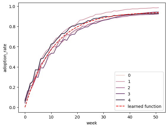
Prediction is easy as well, and similar to above, all we have to do is prepare our test data and pass it to the predict function as we would for many other model libraries. Below is an example of training on a set of curves and predicting on the same timeline to ensure that we have learned the relationship correctly:

Because (IMO) the point of using Bayesian models is to take advantage of their ability to capture uncertainty, I augmented the predict function to take in an alpha parameter, which is used to generate credible intervals for predictions as well, and they are output along the median predictions in the output. Below is an example using an alpha of 0.9 with the same dataset as before:

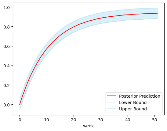
It’s as easy as that!

Saving/Loading

Like other ML libraries, we often want to save our model for prediction at another time, and I have implemented save_trace and load_trace functions accordingly to facilitate this. As long as we reference the same config file for model creation, we can load a saved trace and get straight to prediction.

trace_file_path = 'trace.pkl'
model.save_trace(trace_file_path)

new_model = PymcModel(config)
new_model.load_trace(trace_file_path)

new_model.predict(X_test)

Creating Config with Posteriors as Priors

One potential use case I’ve found interesting is to learn from a established product/geo and apply the posteriors as priors to a new area. Rather than manually updating configs, I added an export_trained_config function that updates the priors in the original config with posterior means and saves it to an output file. Similar to above, we could consume this updated config file to create a new model object.

Periodic Retraining

One last use case I thought might be interesting to showcase is the ability to call the fit function on multiple sets of data. In the following example, I fitted a model to the adoption rate curves we saw above, exported the trained config file, created a new model with it as priors, and finally did a series of repeated fitting on data in chunks of 4 weeks to see how the predicted curve developed over time. The performance at the beginning isn’t great, as it overpredicts the curve steepness at first, but with the noise early on, it’s not totally unreasonable. Either way, it definitely gets more confident over time as it gains more observed data and stabilizes after a few months of data.

Feedback

While this is definitely a work in progress, I would love for you to check out the repo and the example walkthrough notebook that I used to generate these plots and examples.

If you have any feedback of things you would change, would add or even any thoughts of it something like this is needed at all, I would love to hear from you at my email or github in issues/PRs!