


Predictions As Confidence
As you may already know, classification problems in machine learning commonly (though not always) use algorithms that output a predicted probability value that can be used to gauge confidence in how sure your model is that the input belongs to one particular class.
Setting Probability Thresholds
In introductory ML courses, a default value of 0.50 is usually used as the prediction cutoff for making the decision to consider a binary classification output as either positive or negative class, but in industry, selecting the right cutoff threshold is critical to making good business decisions.
If the cost associated with false negatives is large, it may be optimal to use a lower probability decision threshold to capture more positive users at the expense of including more false positives, and vice versa, and the data scientist will work with the business units to balance this tradeoff in order to minimize cost or maximize the benefit. Ultimately, this causes the predictions to act more as a ranking system for applications that require binary classifications as the final output than actually leveraging the values themselves.
Interpretation Problems
Model As Ranking
This model-as-ranking system works fine in many situations, but what happens when your predicted probability does not actually represent the probability and the business unit consuming your predictions assumes that they are? An example of this might be the likelihood of conversion for a given user, which is then multiplied by potential LTV to prioritize leads for a sales organization based on expected ROI. If a model tends to over/underestimate probabilities at the lower/upper ends of the predicted probability spectrum respctively (as random forest models have been known to do), you can end up spending effort on individuals who are less worth the team’s time, wasting resources and potentially losing revenue.
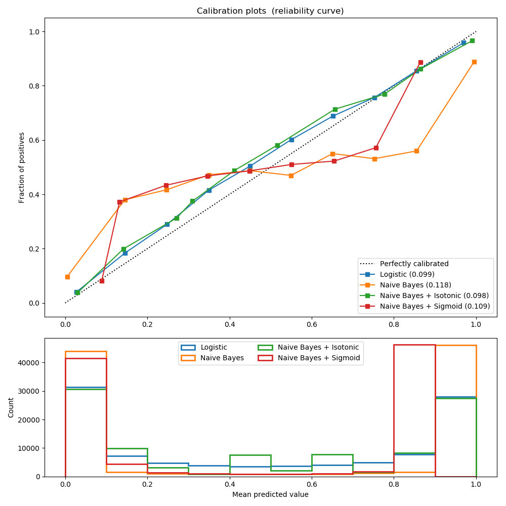
Scikit-learn has a great overview on some common algorithms that result in biased predicted probabilities. I’ve taken the liberty of displaying the chart from that overview here. Visit this link to get the full code used to generate the plot or just look at the documentation for the sklearn.calibration.calibration_curve function
Parallel Model Consumption
Additionally, models can be used in conjunction with one another to provide targets in context. Going back to our expected LTV example, a business may have separate conversion likelihood models for different segments of their customer population, with every user being assigned a conversion probability from a single model. If not all models produce well-calibrated predicted probabilities, one could end up dominating the others while still having good metrics when considered individually.
AUROC Can Be Misleading
One common performance metric that is used to measure the effectiveness of the model across the range of predicted probabilities is the area under the receiving operating characteristic (ROC) curve. In case you aren’t familiar with the ROC curve, it is a plot of the model’s true positive rate vs the false positive rate as the probability is varied from 0 to 1, and as such, it is considered more of a robust metric than accuracy alone in cases where classes are imbalanced or the cost of true/false positives are unknown as of yet.
While it is a good metric, it is not sensitive to the absolute value of the predicted probabilities, only the performance at every probability point. If all of the predicted probabilities are multiplied by a constant, the value of the AUROC does not change, which may mislead the modeler into believing their probabilities are good to use, while in fact, they are consistently over/underestimating the results.
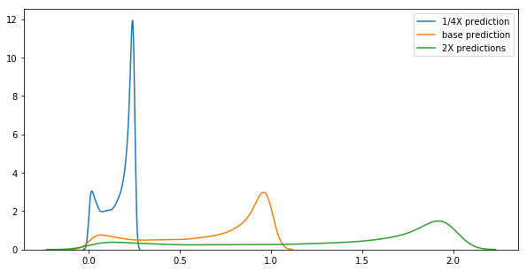
For example, the three predicted probability density distributions below are just scaled versions of the output from the same model. Their distributions are obviously very different from one another, but because they are scaled by a constant, they all have an equivalent AUROC score.
Validation with Additional Scoring Methods
As with most modeling, it’s impossible to represent overall performance with a single number, and if you have concerns about validating probability calibration, it seems wise to include additional scores alongside AUROC that are more representative of actual differences in calibration such as log loss or the brier score.
Log loss is a common loss function, but brier score was new to me, and according to wikipedia “can be thought of as… a measure of the ‘calibration’ of a set of probabilistic predictions”. It essentially is the average squared difference between the probability that was forecast and the actual outcome of the event. This makes its interpretation analogous to the RMSE for regression problems, and does take into account the scale of the predictions.
Sampling Bias
Many problems have imbalanced datasets in terms of the target variable with a significant portion of the records belonging to one class. Various techniques have been developed to counteract these problem, including oversampling the minority class, downsampling the majority class and generating synthetic samples from the minority class to closer achieve class number parity. However, these techniques can result in increased AUROC scores while biasing the predicted probabilities to be less calibrated to actual.
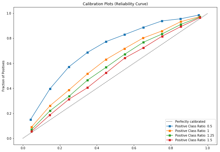
Here is an example of how a generally well calibrated classifier (Logistic Regression) can be biased depending upon the ratio of the positive to negative class in the training dataset:
Further Research
Scikit-learn has implemented the CalibratedClassifierCV class to adjust your classifiers to be more calibrated either during training, or to adjust the predictions by calibrating the classifier post-training.
It has two options for doing so: